This is the third instalment in the Beginners Guide to TShark Series. Please find the first and second instalments below.

• Beginners Guide to TShark (Part 1)
• Beginners Guide to TShark (Part 2)

TL; DR

In this part, we will understand the reporting functionalities and some additional tricks that we found while tinkering with TShark.

Table of Content

• Version Information
• Reporting Options
  • Column Formats
  • Decodes
  • Dissector Tables
  • Elastic Mapping
  • Field Count
  • Fields
  • Fundamental Types
  • Heuristic Decodes
  • Plugins
  • Protocols
  • Values
  • Preferences
  • Folders
• PyShark
  • Installation
  • Live Capture
  • Pretty Representation
  • Captured Length Field
  • Layers, Src and Dst Fields
• Promisc Capture

Version Information

Let’s begin with the very simple command so that we can understand and correlate that all the practicals performed during this article and the previous articles are of the version depicted in the image given below. This parameter prints the Version information of the installed TShark.

tshark -v

Reporting Options

During any Network capture or investigation, there is a dire need of the reports so that we can share the findings with the team as well as superiors and have a validated proof of any activity inside the network. For the same reasons, TShark has given us a beautiful option (-G). This option will make the TShark print a list of several types of reports that can be generated. Official Manual of TShark used the word Glossaries for describing the types of reports.

tshark -G help

Column Formats

From our previous practicals, we saw that we have the Column Formats option available in the reporting section of TShark. To explore its contents, we ran the command as shown in the image given below. We see that it prints a list of wildcards that could be used while generating a report. We have the VLAN id, Date, Time, Destination Address, Destination Port, Packet Length, Protocol, etc.

tshark -G column-formats

Decodes

This option generates 3 Fields related to Layers as well as the protocol decoded. There is a restriction enforced for one record per line with this option. The first field that has the “s1ap.proc.sout” tells us the layer type of the network packets. Followed by that we have the value of selector in decimal format. At last, we have the decoding that was performed on the capture. We used the head command as the output was rather big to fit in the screenshot.

tshark -G decodes | head

Dissector Tables

Most of the users reading this article are already familiar with the concept of Dissector. If not, in simple words Dissector is simply a protocol parser. The output generated by this option consists of 6 fields. Starting from the Dissector Table Name then the name is used for the dissector table in the GUI format. Next, we have the type and the base for the display and the Protocol Name. Lastly, we have the decode as a format.

Elastic Mapping

Mapping is the outline of the documents stored in the index. Elasticsearch supports different data types for the fields in a document. The elastic-mapping option of the TShark prints out the data stored inside the ElasticSearch mapping file. Due to a large amount of data getting printed, we decided to use the head command as well.

tshark -G elastic-mapping | head

Field Count

There are times in a network trace, where we need to get the count of the header fields travelling at any moment. In such scenarios, TShark got our back. With the fieldcount option, we can print the number of header fields with ease. As we can observe in the image given below that we have 2522 protocols and 215000 fields were pre-allocated.

tshark -G fieldcount

Fields

TShark can also get us the contents of the registration database. The output generated by this option is not as easy to interpret as the others. For some users, they can use any other parsing tool for generating a better output. Each record in the output is a protocol or a header file. This can be differentiated by the First field of the record. If the Field is P then it is a Protocol and if it is F then it’s a header field. In the case of the Protocols, we have 2 more fields. One tells us about the Protocol and other fields show the abbreviation used for the said protocol. In the case of Header, the facts are a little different. We have 7 more fields. We have the Descriptive Name, Abbreviation, Type, Parent Protocol Abbreviation, Base for Display, Bitmask, Blurb Describing Field, etc.

tshark -G fields | head

Fundamental Types

TShark also helps us generate a report centralized around the fundamental types of network protocol. This is abbreviated as ftype. This type of report consists of only 2 fields. One for the FTYPE and other for its description.

tshark -G ftypes

Heuristic Decodes

Sorting the Dissectors based on the heuristic decodes is one of the things that need to be easily and readily available. For the same reason, we have the option of heuristic decodes in TShark. This option prints all the heuristic decodes which are currently installed. It consists of 3 fields. First, one representing the underlying dissector, the second one representing the name of the heuristic decoded and the last one tells about the status of the heuristic. It will be T in case it is heuristics and F otherwise.

tshark -G heuristic-decodes

Plugins

Plugins are a very important kind of option that was integrated with Tshark Reporting options. As the name states it prints the name of all the plugins that are installed. The field that this report consists of is made of the Plugin Library, Plugin Version, Plugin Type and the path where the plugin is located.

tshark –G plugins

Protocols

If the users want to know the details about the protocols that are recorded in the registration database then, they can use the protocols parameter. This output is also a bit less readable so that the user can take the help of any third party tool to beautify the report. This parameter prints the data in 3 fields. We have the protocol name, short name, and the filter name.

tshark –G protocols | head

Values

Let’s talk about the values report. It consists of value strings, range strings, true/false strings. There are three types of records available here. The first field can consist of one of these three characters representing the following:

V: Value Strings

R: Range Strings

T: True/False Strings

Moreover, in the value strings, we have the field abbreviation, integer value, and the string. In the range strings, we have the same values except it holds the lower bound and upper bound values.

tshark –G values | head

Preferences

In case the user requires to revise the current preferences that are configured on the system, they can use the currentprefs options to read the preference saved in the file.

tshark –G currentprefs | head

Folders

Suppose the user wants to manually change the configurations or get the program information or want to take a look at the lua configuration or some other important files. The users need the path of those files to take a peek at them. Here the folders option comes a little handy.

tshark –G folders

Since we talked so extensively about TShark, It won’t be justice if we won’t talk about the tool that is heavily dependent on the data from TShark. Let’s talk about PyShark.

PyShark

It is essentially a wrapper that is based on Python. Its functionality is that allows the python packet parsing using the TShark dissectors. Many tools do the same job more or less but the difference is that this tool can export XMLs to use its parsing. You can read more about it from its GitHub page.

Installation

As the PyShark was developed using Python 3 and we don’t Python 3 installed on our machine. We installed Python3 as shown in the image given below.

apt install python3

PyShark is available through the pip. But we don’t have the pip for python 3 so we need to install it as well.

apt install python3-pip

Since we have the python3 with pip we will install pyshark using pip command. You can also install PyShark by cloning the git and running the setup.

pip3 install pyshark

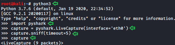
Live Capture

Now to get started, we need the python interpreter. To get this we write python3 and press enter. Now that we have the interpreter, the very first thing that we plan on doing is importing PyShark. Then we define network interface for the capture. Followed by that we will define the value of the timeout parameter for the capture.sniff function. At last, we will begin the capture. Here we can see that in the timeframe that we provided PyShark captured 9 packets.

python3
import pyshark
capture = pyshark.LiveCapture(interface=’eth0’)
capture.sniff(timeout=5)
capture

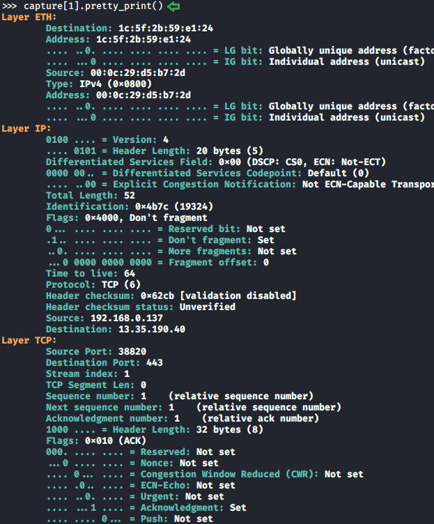
Pretty Representation

There are multiple ways in which PyShark can represent data inside the captured packet. In the previous practical, we captured 9 packets. Let’s take a look at the first packet that was captured with PyShark. Here we can see that we have a layer-wise analysis with the ETH Layer, IP Layer, and the TCP Layer. 

capture[1].pretty_print()

Captured Length Field

In our capture, we saw some data that can consist of multiple attributes. These attributes need fields to get stored. To explore this field, we will be using the dir function in Python. We took the packet and then defined the variable named pkt with the value of that packet and saved it. Then using the dir function we saw explored the fields inside that particular capture. Here we can see that we have the pretty_print function which we used in the previous practical. We also have one field called captured_length to read into that we will write the name of the variable followed by the name of the field with a period (.) in between as depicted in the image below.    

capture[2]
pkt = capture[2]
pkt
dir(pkt)
pkt.captured_length

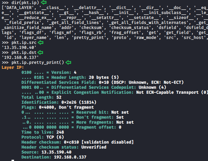
Layers, Src and Dst Fields

As we listed the fields in the previous step we saw that we have another field named layers. We read its contents as we did earlier to find out that we have 3 layers in this capture. Now to look into the individual layer, we need to get the fields of that individual layer. For that, we will again use the dir function. We used the dir function on the ETH layer as shown in the image given below. We observe that we have a field named src which means source, dst which means destination. We checked the value on those fields to find the physical address of the source and destination respectively.  

pkt.layers
pkt.eth.src
pkt.eth.dst
pkt.eth.type

For our next step, we need the fields of the IP packet. We used the dir function on the IP layer and then we use src and dst fields here on this layer. We see that we have the IP Address as this is the IP layer. As the Ethernet layer works on the MAC Addresses they store the MAC Addresses of the Source and the Destination which changes when we come to the IP Layer.

dir(pkt.ip)
pkt.ip.src
pkt.ip.dst
pkt.ip.pretty_print()

Similarly, we can use the dir function and the field’s value on any layer of the capture. This makes the investigation of the capture quite easier.

Promisc Capture

In previous articles we learned about the promisc mode that means that a network interface card will pass all frames received up to the operating system for processing, versus the traditional mode of operation wherein only frames destined for the NIC’s MAC address or a broadcast address will be passed up to the OS. Generally, promiscuous mode is used to “sniff” all traffic on the wire. But we got stuck when we configured the network interface card to work on promisc mode. So while capturing traffic on TShark we can switch between the normal capture and the promisc capture using the –p parameter as shown in the image given below.

ifconfig eth0 promisc
ifconfig eth0
tshark -i eth0 -c 10
tshark -i eth0 -c  10 -p

Author: Shubham Sharma is a Pentester, Cybersecurity Researcher and Enthusiast, contact here.